Bearings are used under various operating conditions; however, in most cases, bearings receive radial and axial load combined, while the load magnitude fluctuates during operation.
Therefore, it is impossible to directly compare the actual load and basic dynamic load rating.
The two are compared by replacing the loads applied to the shaft center with one of a constant magnitude and in a specific direction, that yields the same bearing service life as under actual load and rotational speed.
This theoretical load is referred to as the dynamic equivalent load (P).
Calculation of dynamic equivalent load
Dynamic equivalent loads for radial bearings and thrust bearings (α≠90°) which receive a combined load of a constant magnitude in a specific direction can be calculated using the following equation,

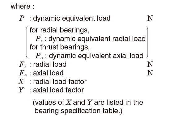
- When Fa/Fr≦e for single-row radial bearings, it is taken that X=1, and Y=0.
Hence, the dynamic equivalent load rating is Pr=Fr.
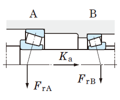
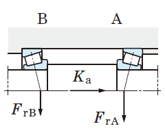
Values of e, which designates the limit of Fa/Fr, are listed in the bearing specification table. - For single-row angular contact ball bearings and tapered roller bearings, axial component forces (Fac) are generated as shown in Fig. 5-11, therefore a pair of bearings is arranged face-to-face or back-to-back.
The axial component force can be calculated using the following equation.
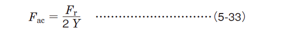
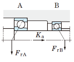
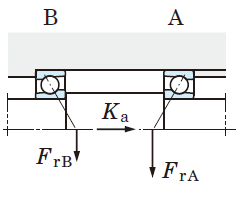
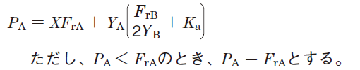
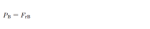
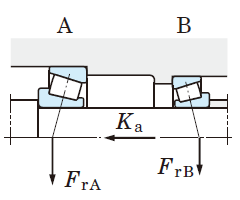
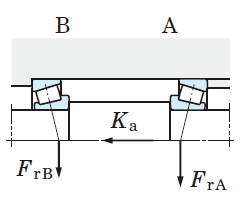
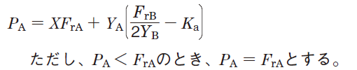
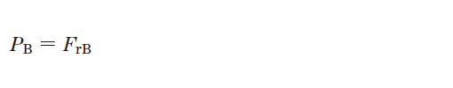
Table 5-9 describes the calculation of the dynamic equivalent load when radial loads and external axial loads (Ka) are applied to bearings.
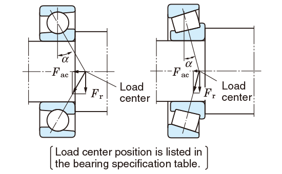
Fig. 5-11 Axial component force
- For thrust ball bearings with contact angle α=90°, to which an axial load is applied, Pa=Fa.
- The dynamic equivalent load of spherical thrust roller bearing can be calculated using the following equation.

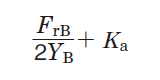
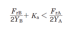
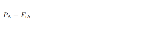
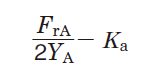
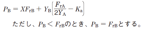
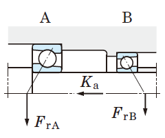
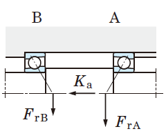
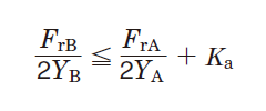
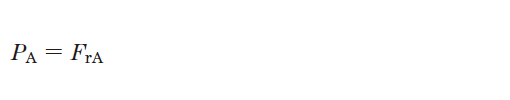
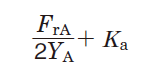
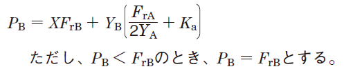
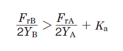
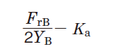
Table 5-9 Dynamic equivalent load calculation : when a pair of single-row angular contact ball bearings or tapered roller bearings is arranged face-to-face or back-to-back.
| Paired mounting | Loading condition | Bearing | Axial load | Dynamic equivalent load | |
|---|---|---|---|---|---|
| Back-to-back arrangement | Face-to-face arrangement | ||||
 |
 |
|
Bearing A |
 |
 |
| Bearing B | - |
 |
|||
 |
 |
 |
Bearing A | - |
 |
| Bearing B |
 |
 |
|||
 |
 |
 |
Bearing A | - |
 |
| Bearing B |
 |
 |
|||
 |
 |
 |
Bearing A |
 |
 |
| Bearing B | - |
 |
|||
[Remarks]
1. These equations can be used when internal clearance and preload during operation are zero.
2. Radial load is treated as positive in the calculation, if it is applied in a direction opposite that shown in Fig. in Table 5-9.
5-4-2 Mean dynamic equivalent load
When load magnitude or direction varies, it is necessary to calculate the mean dynamic equivalent load, which provides the same length of bearing service life as that under the actual load fluctuation.
The mean dynamic equivalent load (Pm) under different load fluctuations is described using Graphs (1) to (4).
As shown in Graph (5), the mean dynamic equivalent load under stationary and rotating load applied simultaneously, can be obtained using equation (5-39).
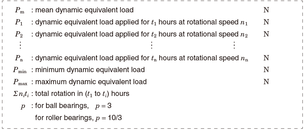
Symbols for Graphs (1) to (4)
[Reference] Mean rotational speed nm can be calculated using the following equation :

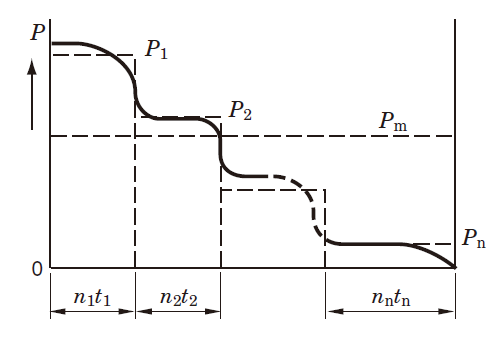
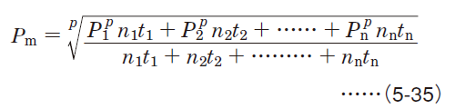
(1) Staged fluctuation
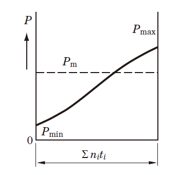
(2) Stageless fluctuation
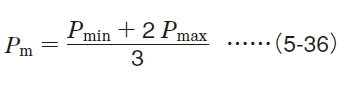
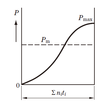
(3) Fluctuation forming sine curve
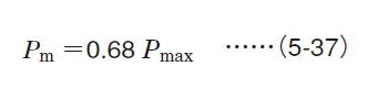
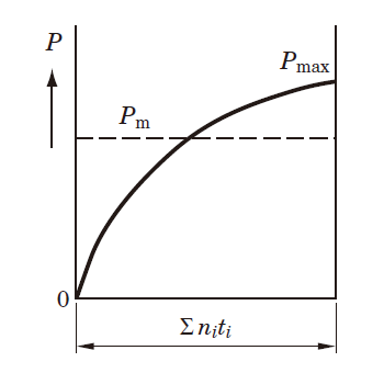
(4) Fluctuation forming sine curve (upper half of sine curve)
(5) Stationary load and rotating load acting simultaneously
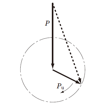
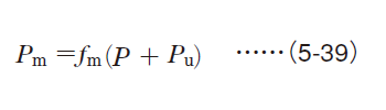
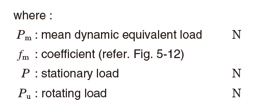
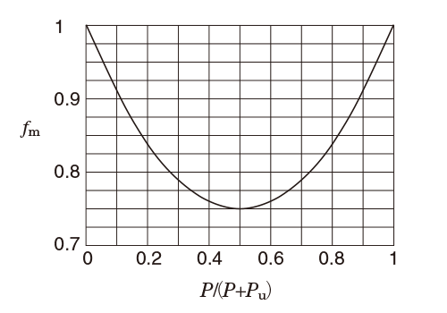
Fig. 5-12 Coefficient ƒm